M&M Binomial

This uses data gathered from the M&M Activity.

Let's begin this with a thought experiment.  Imagine you have the job of filling bags with M&Ms.  One might imagine that there is a huge bin that has been filled with M&Ms and that you are just parcelling them out into the bags.

There is a mountain of M&Ms and a certain proportion of these are red, orange, yellow, green, blue, and brown.  The number is so large that the act of choosing, say, a red M&M on one trial does not appreciably reduce the probability of getting one on the next trial.  All of this argues that, if one is interested in particular colors, each trial is a Bernoulli Trial with a fixed probability of success.

Each M&M is about the same weight and you are aiming to fill your bag to at least a certain weight but not more than one M&M more than that.  This results in the bags having a small variation in number of M&Ms per bag.  All of this means that we have a, more or less, fixed number of M&Ms per bag.

We combine these two observations, and what we have looks astonishingly like a Binomial Experiment.

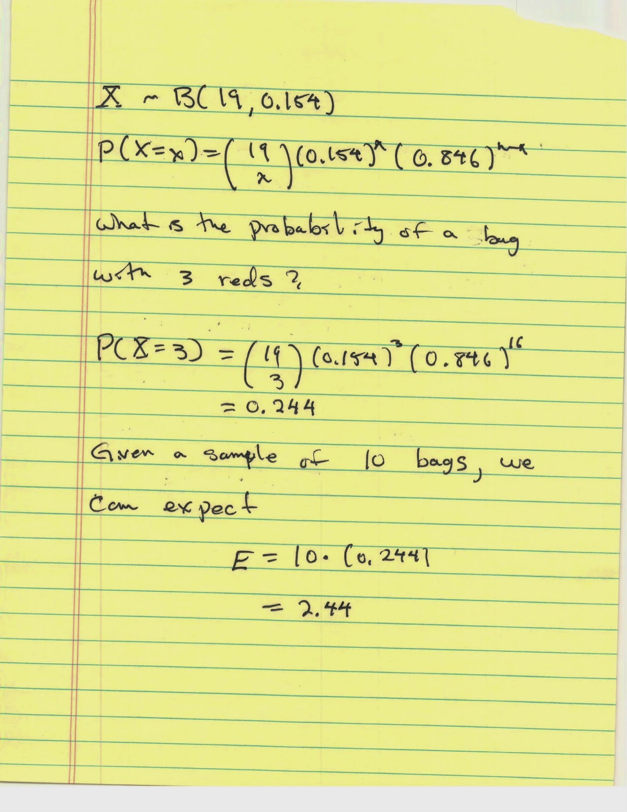
Using a sample of 10 bags of Plain M&Ms, I investigated whether they did in fact follow the binomial distribution for red M&Ms.  This sample contained a total of 182 M&Ms of which 28 were red.  This yields a proportion p=0.154 of red M&Ms. The ten bags contained from 17 to 19 each. I therefore chose to set n=19.

Given those, I used my data to create a frequency table.  In the table below, the first column is the possible number of successes for a binomial experiment with 19 trials, that is to say the numbers from 0 to 19 inclusive; keeping with standard notation, that column is labeled x.  The second column is the number of bags that had that many red M&Ms.  As we are setting up do to a chi square test to see if the binomial model fits, we have labeled the frequency column with an O.

x	O
0	1
1	2
2	2
3	0
4	4
5	0
6	1
7	0
8	0
9	0
10	0
11	0
12	0
13	0
14	0
15	0
16	0
17	0
18	0
19	0

We ask the question of how well this fits with the expectations of the binomial distribution B(19,0.154).  I do the sample calculation for x=3 below:

Putting this calculation into a spread sheet, I obtain:

n	O	E
0	1	0.42
1	2	1.45
2	2	2.36
3	0	2.44
4	4	1.77
5	0	0.97
6	1	0.41
7	0	0.14
8	0	0.04
9	0	0.01
10	0	0.00
11	0	0.00
12	0	0.00
13	0	0.00
14	0	0.00
15	0	0.00
16	0	0.00
17	0	0.00
18	0	0.00
19	0	0.00

We can then compare the values of the O and the E columns by using the (O-E)^2/E measure.  The results are in the table below:

n	O	E	(O-E)^3/E
0	1	0.42	0.81
1	2	1.45	0.21
2	2	2.36	0.06
3	0	2.44	2.44
4	4	1.77	2.80
5	0	0.97	0.97
6	1	0.41	0.85
7	0	0.14	0.14
8	0	0.04	0.04
9	0	0.01	0.01
10	0	0.00	0.00
11	0	0.00	0.00
12	0	0.00	0.00
13	0	0.00	0.00
14	0	0.00	0.00
15	0	0.00	0.00
16	0	0.00	0.00
17	0	0.00	0.00
18	0	0.00	0.00
19	0	0.00	0.00

Note that the sum of the (O-E)^2/E column is 8.32.  The critical number for the chi square test for this is 30.14.  This is the table look up with 19 degrees of freedom and a significance level of 0.05.

As 8.32 is not larger than 30.14, we cannot reject the null hypothesis of the chi square test.  The null hypothesis is that the model fits.  We've no proven that it is binomial, but we can say that our data is not inconsistent with the binomial distribution B(19, 0.154).

Do this test with the data you collected from the M&M Activity.