Lines in Pleasant Places

By Bobby Neal Winters

Lord, you alone are my portion and my cup;

   you make my lot secure.

The boundary lines have fallen for me in pleasant places;

   surely I have a delightful inheritance.

I will praise the Lord, who counsels me;

   even at night my heart instructs me.

--Psalms 16:5-7, NIV

It is rumored that deep within the Ozarks there is a place where those interested go to learn the art of making moonshine.  It is called the Moonshine Academy.  Every year a new class of students enter the academy, but not everyone decides to come back the following year.  The proprietors of the Academy are concerned about this because their aim is spread the art of moonshine making as far and wide as possible.  Those who leave the Academy tend to become Revenuers. They would like to know whether there might be a way to tell ahead of time which of their new students might be at risk of becoming Revenuers.

When each student comes to MA, a record is made of the length of their beards and the number of missing teeth.  The proprietors wish to make predictions based on those two characteristics, having noted that those who have become successful as moonshiners have certain standards with respect to them.  

Some Math

There are two groups, those who succeed and those who don’t. Call the group that succeeds the Elect and denote them by E. We will denote the rest by R, for Revenuer.   We will begin the discussion by assuming a simpler situation than what we have and supposing there is only one characteristic or, to use the standard nomenclature, random variable to measure.  Call it X.

Random variables are functions that take values on populations.  We will write X|E for X restricted only to members of the Elect and X|R for X restricted only to revenuers.  We hope that we won’t be piling on too much notation if we let mean(X|E) denote the mean of X for members of the Elect and let mean(X|R) be the mean of X for members of the Revenuers.

Suppose that we find mean(X|R)

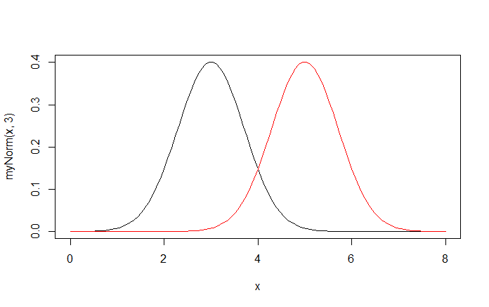
In the figure, we note mean(X|R)=3 and mean(X|E)=5.

In our dreams, we want a magic number C (for cutoff). Say a student named Maynard walks in and his random variable is X(Maynard).  We would like to be able to say that if X(Maynard)> C, then Maynard would be one of the Elect and if X(Maynard)

As Yogi Berra said, “Predicting is hard, especially about the future.” In making making a prediction about Maynard’s future, using only the value of X(Maynard), a procedure would be to simply let this magic number C be the midpoint between mean(X|E) and mean(X|R), respectively, and predicting using the method described above, with the realization that you are going to be wrong some of the time.

This is the same as saying predicting Maynard to be in the group E if X(Maynard) is closer to the mean of X on E than it is to the mean of X on R and to be in R otherwise.

Some More Math

Recall that the folks at the Moonshine Academy had two random variables they kept on each of their students: beard length and number of missing teething.  Mathematicians like to abstract, so we can think of each of the students at MA as a point in space and the values of the random variables coordinates for that point.  We can then plot them out on an X-Y axis.  The results might look like those below:

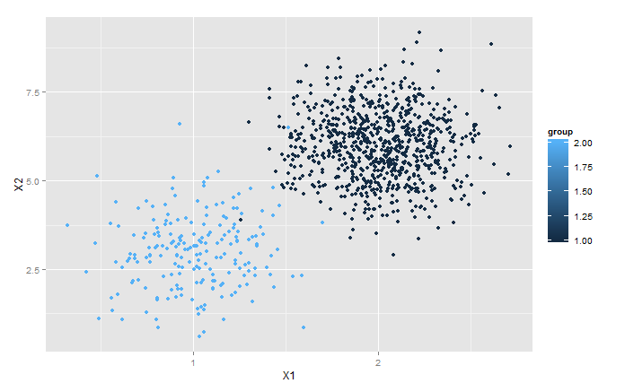
As you see here, the data separates into two groups.  There is one in the lower left hand corner that appears to be centered at about (1,1) and another in the upper right that appears to be centered at about (2,2).

Notice that these two groups are more clearly separated on the 2-dimensional plane than either would be if we simply ignored one of the random variables.   Ignoring the vertical component, for example, would cause collisions between quite a few members of the two groups and there would be considerably more overlap between the 1-dimensional projections of the two groups.

If only there were some way to rotate the picture so that the line connecting the centers of these two groups so that it aligned with the horizontal.

Even More Math

There is, in fact, a way to perform such a rotation. One could apply a rotation matrix.  That’s right, matrices have uses beyond just things to be row-reduced to solve linear systems of equation.  Indeed, there real purpose is that of geometric transformation.  If you multiply a line by a matrix (by which I mean each point on that line), the result will be either a line or a single point.  If the determinant of that matrix is not zero, then the result will always be a line.  What is more, if you multiply a parallelogram of area A by a matrix of determinant D, you will get a parallelogram of area DxA.  And that’s what determinants are all about. Pretty cool if you ask me.

In this particular case, we probably could get away with multiplying by a rotation matrix that we pick by inspection.  However, there is a standard procedure, which we will describe in excruciating detail later, wherein we can obtain the matrix.  At this point, let’s pretend we’ve gone gone through it and obtained a matrix M.  We then take the a point with coordinates (x1,x2) and put it in the row matrix Y=[x1, x2].  We can then obtain the coordinates of the transformed point as YxM, using matrix multiplication.   Applying this to every point gives the picture below:

Note that these two blobs are fairly well separated. One could simply forget about the vertical component  and project the points onto the horizontal axis in order to go through the procedure described at the first of this article.

I like to think of the groups in the above picture as spongy clouds.  They have centers that you can obtain simply by taking the averages of all the of coordinates of each.  The centers of the groups above are exactly the same as the rotated versions of the  centers of the groups in the previous picture.

The Process from Thirty-thousand Feet

I am now going to give you the big picture by telling a few lies.  Later in the article, if you are still awake, I will provide as many details as I can.

Suppose that a new student comes to seek admission to the Moonshine Academy.  The folks at the Admissions Office will measure his beard and count the number of teeth his as missing. (Sometimes they will count the number of teeth he has and subtract that from 32 because it is easier, but I digress.)   They will then measure the distance between that point and the centers of the two groups.  The student will be associated with the group to whose center he is closer.  That is if he is closer to the center of the Elect group he will be predicted to be Elect; if he is closer to the center of the Revenuer group he will be predicted to be a Revenuer.

The word predicted is very important in the paragraph above.  Predictions can be wrong.  Indeed, even when you use a procedure on data where you know the answers, some of the predictions will be wrong.  For example, for the data above we get the following table:

	Predicted
Actual	E	R
E	799*	1
R	2	198*

This says that my model predicted 801 (799 + 2) be in the Elect; of these 799 were but two actually flunked out and became Revenuers.  It predicted 199 (1+198) to become Revenuers.  The model was right in 997 (799*+198*) of its predictions for its founding data. (That is why those numbers are marked with a *.)   These are incredibly good results and this will certainly not be the case with all data sets.

What Happened to the Rotation?

You might have noticed that I’d made a big deal about rotating the matrices to better see how nicely separated the groups were along the horizontal axis, but when I described the process the groups weren’t actually rotated.  This is because you don’t have to rotate for the test. The rotation does not change the distances.  What would be the closest center in the rotated picture would be closest in the unrotated picture.

However, once the initial test is run and you want to make predictions about candidates for next year it is more convenient to have a formula.  For the data above the formula would be: f(bl,mt)=0.982*bl+0.188*mt. Here, bl=beard length and mt=missing teeth.  It is easier to determine whether f(bl,mt)>2.330 than it would be to calculate the distance to each of the centers of the groups.  

And, as a student who would want to look good with respect to these standards, it is easier to tell that you’d be best advised to spend your time growing your beard as opposed to pulling your teeth.

How Do We Get That Formula?

To get to that formula, we must enter into the jungle of matrices where many enter and few emerge unchanged.

The first matrix I want to introduce you to is the covariant matrix. There is far more to know about it than what I am going to tell you.  This is how you get a covariant matrix.  Let X be a matrix each of whose columns are values of a random variable.  So column one will contain the beard length of each of our students and column two will contain the number of missing teeth of the same student. If you have more random variables to study, you will have more columns.  For us, with the beard lengths and the missing teeth of 1000 students, we have X as a 1000x2 matrix.

Now, calculate the mean of each column and subtract that number from each of the columns.  Call this new matrix Y. So each element of Y will be the difference between the value of a particular random value for a particular student and the mean of that random variable for all the students.  Now the covariant matrix of X, cov(X), is transpose(Y)*Y.  For us it will be a 2x2 matrix.  Note that cov(X) is symmetric; it is important.

Now, forget about this particular matrix because we are not going to use it, but remember how we got it.

Let XE be the data for the Elect and let XR be the data for the Revenuers. Let pE be the proportion of the data that is from the Elect and pR be the proportion from the Revenuers.  Let Sw=pE*cov(XE)+pR*cov(XR). Note that Sw is symmetric; it is important.

Now remember that first matrix X, the one I told you to forget about.  We are going to fix it.  Instead of being the value of the random variable minus the mean whole column, let it mean of the column for the data group minus the mean of the whole column.  That is to say if the student from row i is in the Elect, his entry in the Beard Length column will be the average beard length for the Elect minus the average beard length for everybody.  Then Sb=cov(X).  Note that Sb is a symmetric matrix; this is important.

Now let M=inverse(Sw)*Sb.  Inverse(Sw) is symmetric so M is symmetric.  This is important. Write it on your hand with a sharpie.

We are about to digress.

Eigen What?

A discussion of eigenvalues and eigenvectors would take us too far afield.  One or more of us would be dead by the time I finished.  Suffice it to say that the theory is beautiful in the same way the Arctic is: The beauty is real, but seeing it face to face comes at a cost.

It is enough for us to know the following. If M is a symmetric matrix, and it is, then there is a matrix P and a diagonal matrix D such that M=transpose(P)*D*P.  Furthermore, the matrix P will consist of the eigenvectors of M, whatever the hell they are, and the diagonal entries of D will be the eigenvalues of M, whatever the hell they are.  Take the eigenvector corresponding to the eigenvalue of largest absolute value and multiply it by the coordinates of the student, and you have your formula.  For us that is [bl , mt] * transpose([0.982, 0.188]).  To get the critical point C, one applies this formula to the midpoints of each of the groups, and takes the average of the two.

References

“Linear Discriminant Analysis-A Brief Tutorial,”  S. Balakrishnama and A. Ganapathiraju, Institute for Signal and Information Processing

Discriminant Analysis, William. R. Kleka, A Sage University Paper, Series: Quantitative Applications in the Social Sciences, 1980

Cora Layton

Cora Layton

By Bobby Neal Winters

Math folks, like everyone else, enjoy congregating with their own kind from time to time.  By own kind, I mean to say people of similar, if somewhat strange, interests.  We do this at conferences.  Over the years, I’ve attended conferences featuring talks in a variety of mathematical and mathematically-related topics.  Aside from the talks, the real purpose of these conferences is to establish human relationships between real, living human beings.

One problem with this is that it is hard for anyone to envision those of us who practice the arcane mathematical arts as human beings real, living, or any other way.  Nevertheless, I have, over the years, managed to get to know a few of my fellow math-types.  One of these is Cora Layton.

Cora worked for many years at Sutherland State University teaching statistics.  Statistics is not as some people think--including some mathematicians--a branch of mathematics.  It is a proud discipline of its own that uses mathematics.  

Cora had not only taught students, but she’d also done considerable work helping her colleagues in the sciences and social sciences with some of their statistical problems.  

At the last conference, I’d heard she’d retired.  Imagine my surprise at going to a mathematics meeting, looking up, and seeing her there.

“Cora,” I said.  “Is that you?”

Her smile let me know that indeed it was her.

“Well, who else would it be?” she replied coyly, her southern accent so thick and sweet that you could imagine honey dripping from it.

“I’d been told that you had retired,” I said.

“Can we ever really retire?” she asked.  I’ve heard this question asked a lot, mostly in relation to retirement accounts depleted by the stock market crash.

We left the conference and went for a coffee so that we could catch up with each other’s news.

As we sat there with our four-dollar designer coffees, I discovered that she had, in fact, retired from teaching.  However, she’d needed to keep busy and hung out her shingle as a consultant.  Doing this, she was able to stay only a bit busier than she wanted to be.

I said she’d hung out her shingle.  These days a shingle need only consist of a page on the Internet. Being a teacher, I am always on the look for real-life applications for the classes I teach.  I thought that in her new role she would be able to share some.

“So, Cora,” I began my inquiry, “have you run into any interesting problems that I could share with my students?”

Cora smiled.  

“I don’t know that I’d call this a real-life problem,” she said, “but I found it interesting.”

She took a sip of her coffee and related her tale.

At first, most of her work had been a continuation of her role in helping her former colleagues at Sutherland State with their projects.  Then one day she’d been contacted “out of the blue” as they say by a couple of men in their late twenties or early thirties.  

 The first contact had been by e-mail and had looked official enough.  They had given their names as William R. [redacted] and James J. [also redacted] and bottom of the e-mail boldly claimed them to be representatives of the Weather and Atmospheric Cloud Organization, WACO for short.  

Cora was to learn that they were more widely known as Billie Bob and Jimmie Joe. She’d smiled to herself when she read the acronym WACO, figured that they probably hadn’t called in a PR guy on the project, and thought no more about it until she met them.  When she met them she thought the acronym was quite descriptive.

They drove up in a brand new Dodge Ram truck.  It had a shiny, red finish and an even shinier chrome roll-bar.  Sitting in the back was some rather expensive-looking equipment and attached to the roll-bar there was rotating satellite dish.

Billie Bob and Jimmie Joe are tornado chasers.  While there are a good number of respected scientist who chase tornadoes, Billie Bob and Jimmie Joe are not among these.  They consider themselves scientists; they’ve printed up letter head and t-shirts for their WACO organization; they take pictures and have all sorts of fancy equipment; but they fall short in the area of credentials and any sort of grasp of the scientific method.

To their credit, having seen other, more reputable tornado chasers in their activities, they’d come to the decision they wanted to pursue their passion in a more serious way. For this reason they had come to Cora wanting help on a scientific project.  

The idea was this.  They had observed in their various storm chases the devastation that tornadoes wreck on mobile homes.  They are not unique in this observation and had began to wonder whether there was something about mobile home that attracted tornadoes.  They had seen Cora’s page out on the Internet where she helped scientists, and they were scientists that needed her help.

“I almost sent them away,” she told me there at the coffee shop. “I don’t know whether it was because they were about the same age as my grandsons or whether they offered me $1000 up front and I remembered that saying about a fool and his money.  In any case, I am a teacher and I can’t help but teach.”

Cora told them that they needed to collect data.  She said that they needed to visit mobile homes, those which had been hit by tornadoes as well as those that had not.  They should look for things that might reasonably be factors in attracting tornadoes.

She also introduced them to some simple statistical software and had instructed them in the use of it.

“I figured that I ought to be doing something useful for the money,” she said, looking only slightly guilty.

It was much to her surprise when they returned a few weeks later with data.

“They had taken by advice very seriously,” she said.

Billie Bob had noted the presence of car batteries in the yards of many mobile homes.  He’d figured that, as they could be used to produce electricity, it was conceivable this might have some effect on tornado-producing storms.  Jimmie Joe had noted the presence of old tires mounted on rusty wheels in the yards of many of these mobile homes.  He’d wondered whether the roundness of the tires might have anything to do with attracting tornadoes as tornadoes turned in a circle.

They’d made careful counts of these at numerous trailer parks and fed the data into the computer.  What they’d found had astounded them.

“They didn’t find any significant difference in the groups that had been hit by a tornado and the control group,” she said with her lips betraying just a hint of a mischievous smile. “What they did find and what did astound them was a correlation between the number of tires and the number of batteries.  The number of tires is approximately 3.95 the number of car batteries they found.  The 3.95 is accurate plus or minus a margin of error of 0.1.”

I thought about this myself a minute and began to share her smile.

“Did they, by any chance, in the course of collecting data, note the number of old cars up on blocks with their hoods open in these yards?” I asked.

She smiled even more broadly.

“They did not,” she said. “But I did suggest they broaden their study to include the width of satellite dishes and sofas on the front porch.  My sister lives in Florida and it’s been a while since I’ve seen her.  If they do a little more science, I might be able to afford the trip.”