Calculating orbits: Introduction

Introduction

The general problem we will be approaching will be one object orbiting another object in space.  This general language becomes cumbersome, however, so we will us that of a planet orbiting the sun. My philosophy of approach will be to begin with the big picture and to slowly fill in the details of the big picture so that the reader can dismount when a certain level of sophistication is reached without fear of missing anything later that he might have understood, although he is welcome to push on in hope.

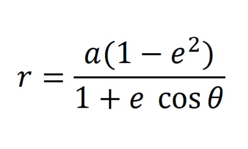
This having been said, if you don’t have an understanding of polar coordinates, now might be a good time to get off the bus.  The basic equation of an orbit in polar coordinates is given by

in polar coordinates.  Recall that polar coordinates are related to rectangular coordinates according to the transformations

In the sequel, as far as orbit calculations are concerned per se we will be tossing aside our familiar $\theta$ in favor of the letter $\nu$ as this has been done by my principal source (Spaceflight Dynamics, William E. Wiesel, Third Edition). (Also note that I’ve opted to use LaTex code for inline variable and jpeg for equations.)

In that case, our equation becomes

This is the equation of an ellipse with semimajor axis $a$ and eccentricity $e$. These are quantities associated with an ellipse that we will explore more fully in a later section.

The angle $\nu$ is measured in a counterclockwise direction from the positive $x$-axis to the ray going from the sun to the planet.  The use of an ellipse for a planetary orbit comes from Kepler’s First Law wherein it is stated that planets move around the sun in an ellipse with the sun at one focus.

Given the equation with all of its constants evaluated, we can find $r$ and the polar coordinates  $( r, \nu)$ will give us the equation of the planet.  This mathematics itself is not hard, but a basic difficulty arises because we wish to know the position in terms of a particular time $t$.  The process of doing this is as follows:

We will compute a number $M$ by the equation $M=nt$, where $n$ is a constant that depends on the physics of the system.  We call $M$ the mean anomaly and we will use it in the following equation:

which is called Kepler’s Equation.  The variable $E$ is called the eccentric anomaly.  While there are series solutions for this equations, they are awkward and it is easily solvable by numerical methods.

Given $E$, we may solve for $\nu$ by the use of the equation

One merely plugs $E$ into the right hand side, takes the arctan of the result, and multiplies by 2.

At this point, the only barrier we have to performing a calculation, assuming we have $a$ and $e$, is determining $M$ whose formula requires the mysterious constant $n$.  We can calculate $n$ by the use of

where $k$ is a physical constant given by

which is known as Kepler’s Third Law.  Here $T$ is the amount of time in takes a planet to complete its orbit around the sun, and $a$, as always is the semimajor axis.

For those of you who are alert and have notice we’ve only referred to Kepler’s First and Third Law.  What about the second?  It is used the the derivation of Kepler’s Equation which we leave to a subsequent section.